


MICROECONOMICS
2.1 Market and revenue curves:

The objective of producers is to earn more and more profit. That depends on the market situation. On the basic of level of competition, number of sellers and purchasers, the market can be classified in the different forms. In different market nature of revenue also differs. In this context, the concept of market and revenue is discussed in the following heads.
2.1.1 Concept
of market:
In ordinary sense, market is a place where sellers and buyers meet together to purchase and sell of goods and services. It is physical place in which commodities are sold or purchased according to negotiation of sellers and buyers. In economics, market refers to the purchase and sells of commodity ad the determination of price. So, market means exchange of goods and services. Sellers and purchasers would be contact with one another. On the basis of competitive situation, market can be classified as perfect completion and imperfect competition.
A. Perfect Competition:
Perfect competition is a market structure which is characterized by a large number of buyers and sellers. Sellers remain as small component in relation to total industry. They cannot affect the price of the product significantly. Similarly, the numbers of buyer are large and individual buyer cannot affect the market significantly. Sellers are price takers, not price makers. The assumptions for the existence of perfect competition are as follows:
1. Large number of buyers and sellers.
2. Freedom of entry and exit of firms.
3. Homogeneous product in the market.
4. Profit maximization goal of the firms.
5. Perfect mobility of factors.
6. Perfect knowledge of market conditions.
7. Absence of transportation costs,
8. Horizontal demand curve.
9. Absence of artificial restrictions
Hence, the perfectly competitive market implies no rivalry among the individual firms to capture the market.
B. Imperfect competition:
Imperfect competition is another form of market. It has several forms such as monopolistic competition, oligopoly, duopoly and monopoly.
(i) Monopolistic competition:
It is the mixture at perfect competition and monopoly market. It is a completive market situation where there are large number sellers and sell heterogeneous goods (close substitute but not identical). Individual firms exercise to control over the price to a smaller to larger degree. Each seller can follow its own price output policy. There is products differentiation the characteristics of monopolistic competition are as follows:
1. Large numbers of sellers and buyers.
2. Product differentiation
3. Free entry and exist of firms.
4. Selling costs
5. PIECE MAKERS
(II) Oligopoly:
Oligopoly is a market structure with a small number o firms. They are mutually interdependent for pricing and output policies. Each firm has considerable market share and control over the price. Oligopoly market can be classified as pure and differentiated, if an oligopoly industry products homogenous product (aluminum, cement, steel, etc), it is called pure or perfect oligopoly. If an oligopoly industry produces heterogeneous products (TV sets, refrigerators, soaps, automobiles, cosmetics, etc), it is called imperfect or differentiated oligopoly. The characteristics of oligopoly are as follows:
1. Small number of sellers
2. Nature of product (Homogeneous of heterogeneous)
3. Interdependence of decision making regarding price and output.
4. Barriers to entry the other firms
5. Non-price competition
6. Selling cost
(iii) Monopoly:
Monopoly is a market, in which there is a single seller of a unique product which has no close substitutes and there is strong barrier to entry in to the product. A monopoly exits when a specific firm of enterprise is only the supplier of a particular commodity. Thus, monopoly is the price- maker. Under monopoly, the distinction between the firm and industry disappears. The average revenue curve or the demand curve always slops downward to the right. The characteristics of monopoly as a follows:
a) Single sellers and large number of buyers.
b) No close substitute for the product.
c) Restriction on the entry of new firms.
d) Downward sloping demand curve.
Difference between perfect competition and monopoly market:
1. Difference in the nature of the product: Under perfect competition, product is homogenous with perfect substitute, whereas under monopoly, unique product with no substitute.
2. Difference in the nature of the demand curve: Under perfect competition, demand curve become horizontal parallel to OX axis whereas under monopoly, demand curve slops downwards to the right.
3. Difference in entry and exit of the firm:
Under perfect competition there is free entry and exit of new firms in to the industry, whereas under monopoly, there are barriers to entry new firm in to the market.
4. Difference in knowledge about the market:
Under perfect competition, seller and buyers both have perfect knowledge about the market, whereas under monopoly both have imperfect knowledge about the market.
5. Difference in profit in the long run:
Under perfect competition, firms earn only normal profit in long run whereas under monopoly, firm earn super normal profit in the long run.
6. Difference in role of government:
Under perfect competition, government doesn’t regulate in the market whereas under monopoly, there is government regulation.
2.1.3 Concept of total revenue, average revenue and marginal revenue:
The objective of producers is to increase the level of profit. It depends on the income and its nature of revenue is discussed in the following heads.
a) Concept of Revenue:
The amount of money a firm receives by selling given quantity of its product is called its revenue. In other words, revenue refers to the receipts obtained by a firm from the sale of certain quantity of a commodity at various prices. There are three concepts of revenue: total revenue, average revenue and magical revenue and average revenue would be different in different forms of market.
(i) Total revenue (TR):
The whole income received by the seller from selling a given amount of product is called total revenue. Total revenue is the total sale of products of a firm by selling a commodity at a given price. In other words, total revenue is the sum of marginal revenue obtained from the sale of different units of goods, if a firm sells 2 units of goods at rs.20; total revenue is 2*20=40. So it is the product between total sold units and per unit price.
Symbolically
TR = P*Q
Where,
P= price
Q=Quantity sold
As we know, total revenue is also the summation of marginal revenue.
Thus,
TR= ∑MR=MR1+MR2+…..+MRn
Where, TR= Total revenue, ∑= summation,
MR1= marginal revenue of 1st unit of output,
MR2= marginal revenue of 2nd unit of output,
MRn= marginal revenue of nth unit of output.
ii) Average revenue (AR)
Average revenue is per unit revenue earned of output sold or average revenue is the average receipts from the sale of certain units of the commodity. It is obtained by diving the TR by the number of units sold. Thus,
AR=TR/Q
Where,
AR=Average revenue
TR=Total revenue
Q=unit sold
When the firm earns total revenue of RS.100(TR) by selling 5 units (Q)of output, the revenue earned per unit of output is 20(100/5). Thus, Rs.20 is the average revenue.
(iii)Marginal revenue
Marginal revenue is the net revenue earned by selling an additional unit of the product or marginal revenue is the additional income made to the TR by selling one more unit of the goods. MR is calculated by dividing the change in total revenue by the change in output. It reflects the rate of change in total revenue with respect to change in quantity sold.
Thus,
Where,
MR = marginal revenue
2.1.3 Derivation of total
revenue, average, revenue and marginal revenue under perfect competition and
monopoly market
The nature of perfect competition and monopoly markets is different because of that the nature of receiving revenue it becomes different. In this regard, the derivation of total revenue and marginal revenue is explained on the following topics.
1. Derivation of total revenue, average revenue, and marginal revenue
perfect competition market.
Perfect communications is a market structure which is characterized by a large number of buyers and seller, each of whose transactions are so simple in relation to total industry that they cannot affect the price of production. Similarly, the number of buyers is also too large that each buyer buys an insignificant part of the total supply and has no control over the market price. Sellers are price takers but not price makers. In this market, homogenous products are sold. The price is determined by supply and demand focuses so unit from one price tends to prevail for the whole industry.
Due to constant price, he average revenue curve is horizontal, parallel to the X axis and the marginal revenue curve coincides with it and the total revenue curve slops straight upward to the right. It is because, under perfect competition, the number firms selling and identical product is very large at constant price. It is shown in the table:

The table shows that the quantity sold increases with constant price. Thus the total revenue increases at the same rate (i.e.20, 40, 60, 80 and 100). The table also depicts that the average and marginal revenue remain constant (i.e. 20) at each increasing level of output. It means AR=MR at each level of output sold. It can also be explained with the following diagram:
In the given diagram, OY axis measures revenue and OX axis measures output. TR is the total revenue curve sloped upward from left to right. Total revenue increases at the same proportion as increase in unit sold. Therefore, total revenue curve slopes upward. AR is the average revenue curve slops horizontal straight line or parallel to the X axis. This indicates that whatever be the change in output, sold average revenue (P) remains constant. It is also firm’s demand curve and it is perfectly elastic. MR is the marginal revenue curve. It also slops horizontally or parallel to the OX axis. MR curve coincides with average revenue curve. It is also remains constant at any level of output sold.
2. Derivation of total revenue, average revenue and marginal revenue
under monopoly:
A monopoly is a market structure characterized by a single seller, selling a unique product in the market. In a monopoly market, the seller doesn’t face competition and no close substitutes. The seller control over the supply of commodity. A monopolistic is price maker and determines the price of product based on the law of demand. In monopoly market, there an inverse relationship between output and price. Hence, the total revenue increases at describing rate. But both average and marginal revenue fall continuously. However, the decreasing rate. But both average and marginal revenue fall continuously. However, the decreasing rate of marginal revenues is greater than average revenue
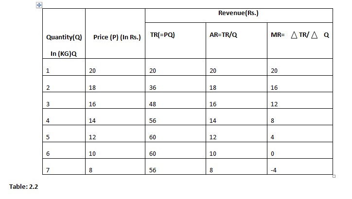
Table: 2.2
As shown in the table, when the seller increases sales unit proportionately from 1 unit to 7 unit at falling prices, total revenue increases in decreasing rate reached at maximum WHEN MARGINAL REVENUE IS 0. After that the total revenue starts to decline due to future fall in price. Consequently, marginal revenue becomes negative (I, e-4). Both average and marginal revenue decrease but the decrease rate of marginal revenue is faster than the decrease rate of average revenue.
In the figure, sold units and revenue are measured along X axis and Y axis respectively. TR is the total revenue curve slopes upward at first then after reached at its maximum point (I e. 60) and finally starts to decline. AR is the average revenue curve slopes downward to the right at each increasing level of output sold. MR is the marginal revenue curve slops downward to the right. It becomes negative when total revenue curve slops downwards. Both AR and MR curves are falling at each increasing level of sold units and MR curve lies below the average revenue curve because, falling rate of MR is greater than AR.
2.2 Cost Curves:
Cost indicates the monetary payments made to the owner of factors of production in the production processes. In the other words, the total expenses incurred on inputs while producing commodity is called cost. The cost of production is important part to analyze a profitability situation of a producer.
2.2.1 Concept of explicit, implicit, fixed, variables and marginal cost
There are different types o costs and may according to change in production processes, regarding this, various concepts of cost are discussed below.
1. Explicit cost:
The cost involving direct payment of money for the purchase of factors of production is known as explicit cost. The payments on account of wages, salaries, utility expenses, interest, and rent, purchase of materials, license fee, insurance fee, insurance premium and depreciation charges are the examples of explicit cost.
2. Implicit cost:
Implicit work is defines as the value of factor inputs owned and used by the firm or the entrepreneur in its own production process. Such cost doesn’t appear in the accounting system. It is similar to opportunity cost. For example, salary of the proprietors to return on the entrepreneur’s own investment. It is not paid in term of money.
3. Fixed cost:
Fixed cost is the expenditure
incurred on the purchase of fixed inputs; fixed cost remains constant to any
changes in output. Even the output is zero, these costs cannot be zero. It
includes interest on capital, insurance fee, property tax, maintenance costs,
and administrative expenses. Etc. they do not very with the level of output.
They remain same regardless of how much it produced by the firm. It is not a
function of output.
4. Variable cost:
It is the cost incurred on the purchase of variable inputs. It is also called prime or direct cost. It includes the payment made to labors, raw materials, fuel, power, transportation fair, etc. variable cost changes with the change in output positively.
5. Marginal cost: Marginal cost is defined as the change in total cost resulting from the one unit change in the quantity produced. It is addition to the total cost caused by producing one more unit of output. In other words, marginal cost is the ratio of change in total cost to the change output which can be expressed as:
MC = TC/ Q
Or, MC=TCn-TCn-1
Where,
MC= marginal cost
TC= change in total cost
Q= change in quantity of output
TCn= total cost of nth unit
TCN-1= TOTAL COST OF (N-1TH) unit
2.2.2 Derivative of short-run cost curves
Short run is a period of time in which at least one factor of production remains constant. In order words, it is period of time within which the firm can increase its output by varying only the variable factors such as purchase of labour, raw material, advertisement cost etc. Such cost various with the change in the level of output. Short run cost includes the total fixed cost (TFC), total variable cost (TVC), total cost (TC), marginal cost (MC), average variable cost( AVC), average fixed cost (AFC) and average cost (AC). They are explained as below.
1. Total fixed cost (TFC)
Total fixed cost is the expenditure incurred on the purchase of fixed inputs. It does not change in output. It includes interest on capital insurance fee, property tax, maintenance costs, administrative expenses etc. They remain the same regardless quantity of production.
2. Total variable cost (TVC)
Total variable cost is the sum of the costs increased on variable factors. Total variable cost changes with change in output positively. If output is increased, total variable cost will be increased and vice- versa. It includes payment made to workers, suppliers of raw material, fuel, power, transportation changes and so on. They do not occur if the production is zero, TVC can be calculated as
TVC =TC-TFC
Where,
TFC= Total fixed cost
TC= total cost
TVC= total variable cost
3. Total cost (TC)
Total cost (TC) is the total sum of total fixed costs and the total variable cost. It also can be derived by multiplanning average cost by the quantity of output.
Symbolically,
TC = TFC + TVC
Or
TC=AC*Q
Short run total cost can be explained with the help of following table:
.jpg)
Table 2.3
In above table, TFC is fixed Rs. 60 regardless not the level of output 0 to 6. TVC is 0 when output is 0 and rises from 100 to 720 as output rises from 1 to 6. At every level of output TC equals TFC plus TVC i.e. (TC= TFC+ TVC). Short run total cost. Fixed cost and variable cost can be diagrammatically explained as follows:
In this diagram, TFC is the total fixed cost curve which is parallel to X axis or output axis. It implies that total fixed cost is always fixed even the later of output is zero. TVC is total variable cost curve. It starts from the zero origin showing that it is zero when output is zero. The shape of TVC is the result of operation of the law of diminishing returns. Up to point T, the TVC curve is concave downwards. It means that TVC increases as the decreasing rate. After point T, TVC is concave upwards showing that TVC increase at the decreasing rate. So the shape of TVC is looked like inverse of alphabet‘s’. TC is the total cost curve. It is also looked like inverse of alphabet‘s’.
4. Average Fixed cost curve (AFC):
The average fixed cost is defined as the fixed cost per unit cost of output and is obtained by diving total fixed cost by units of production. It is expressed as
AFC = TFC/Q
Where, AFC = average fixed cost
TFC = Average fixed cost
Q = Unit of production
Since fixed cost remains unchanged in the short run, with an increase in output, the average fixed cost decreases continuously. Average fixed cost curve thus is a downward sloping to the right.
5. Average Variable cost curve (AVC)
Average variable cost is defined as the variable cost per unit of production and is obtained by dividing the total variable cost by unit’s production. It is expressed as:
AVC= TVC/Q
Where, TVC = total variable cost
AVC= average variable cost
Q= total output produced
The average variable cost initially decreases and after some point begins to increases continuously. At the beginning stage, there would be the proper use of resources, benefit of division of labour and better coordination in production. As a result the cost decreases, but after a limit, the situation becomes reverse. There would be problem in coordination of factors of production, problem in labour management and resources can be misused as a result, the starts to increase gradually.
6. Average total coat curve or average total curve (ATC or AC)
The average total cost is the average cost, it is the cost per unit of production and is obtained by dividing total cost by the number of units of output or it is also the sum of AFC and AVC. It is expresses as:
ATC=TC/Q
OR,
ATC=AFC+AVC
Where,
TC= total cost
Q= total output produced
AFC= Average fixed cost
Single total cost is the sum of total variable cost and total fixed cost, the average total cost is also sum of average variable cost and average fixed cost (i.e. ATC= AVC+ AFC). The concept of short run average cost can be explained with the help of the following table:
.jpg)
Table 2.4
From the above table as the output of a firm increases. AFC falls continuously first rapidly in the beginning and then after falls in low rate. As the output increases, AVC decreases till TVC increases till TVC increases at a diminishing rate and after a certain point it increases when TVC increases at increasing rate. Thus, AVC declines initially and reaches at minimum (i.e. 80) at 3rd units of output. There after it goes on rising. Similarly, as the output increases, ATC decreases initially and reaches at minimum and constant and increases later. Since ATC is the sum of AFC and AQVC, AC falls when AVC and AFC fall at the output range of 1st to 4st unit. After that it increases.
In the figure, AFC is the average fixed cost curve slopes downwards to the right. As output increases, it gets spread over large number of unit of production. Average fixed cost curve is a rectangular hyperbola showing the same level of total fixed cost of total producing all level of output. It is nearer to both the axis but does not touch them.
AVC is the average variable cost curve slopes downward in the beginning, reaches the minimum point M and then after rises upward gradually. It falls at first at due to the operation of increasing returns. But beyond the normal capacity it will rise due to the operation of decreasing returns. Generally, the AVC curve is ‘U’ shaped. Its U shape can be explained in terms of the law of variable proportion.
ATC is the Everest total cost curve. The behavior of average total cost curve depends upon the behavior of average variable cost curve and the average fixed cost curve. ATC is the higher level than either of these costs curves. It, initially decreases, but as output increases, it reaches the minimum point and then rises with the fall in production. Therefore, ATC curve is also a U-shaped.
7. Causes of being ‘U’ shapes of short run average cost curve
Average cost is the outcome of total cost divided by total output. Short run average cost being U shape reflects the law of variable proportions, besides this, there are several factors that help short run average cost curve to be ‘U’ shape. The following are the main reasons of short run average cost curve being ‘U’ shaped:
1. Operation of the law of variable proportions: due to operation of variable proportions SAC curve becomes ‘U’ shaped. At first, SAC declines due to an operation of increasing returns to the variable input and begun to decrease. In this situation, SAC curve rises.
2. Indivisibility of factors:
In short run, some factors of production like machine, an equipment etc. are indivisible. It is impossible to reduced capacity of machines or equipment in order to produce less. Due to this reason, produced of capacity or machine or reduce the per unit cost of output. SO, SAC curve declines at first. But later on there will be diminishing productivity of indivisible factor so SAC curve races. In this way, SAC curve becomes ‘U' shaped.
3. Nature of AFC and AVC
Average fixed cost declines continuously as output increases and average variable is cost curve is also declining at initial stage. So SAC curve is downward sloping initially. Then after SAC reaches its minimum point and finally rises. This is because SAC is the total sum of AFC and AVC.
4. Economic of scale:
Due to the economics of scale, SAC become ‘U’ shaped such economies of scale are technical, economic, managerial economics, marketing economics etc.
8. Marginal cost curve (MC)
Marginal cost may be defined as the change in total cost resulting from other unit change in the quantity produced. It is addition to the total cost cause by producing one more unit of output. IN other words, marginal cost is the ratio of change in total cost to the change in the total output. This can also be defined as the change in total variable cost resulting from a unit change in output, since TFC remains constant at all level of production. It can be expressed as:
MC= TVC/Q
Where,
MC= marginal cost
TC= change in total cost
Q= change in total quantity production
TCU= total cost of nth unit
TCN-1=TOTAL COST OF (N-1TH) unit
TVC = Change in total variable cost
.jpg)
In above table, marginal cost is dependent upon the behavior of TC. When TC increases at diminishing rate, the marginal cost decreases gradually. When TC increases at an increasing rate MC increases, similarly as the output increases, MC falls till TVC increases at an increasing rate and increases and start to increases when TVC increases at a diminishing rate and increases and starts to increase when TVC increases at an increasing rate. It is because MC shows the rate of change in TVC with respect to change in output.
As shown in the figure, MC is the marginal cost curve which is also ‘U’ shape. Since marginal cost is directly dependent upon the behavior of TVC alone. MC is also ‘u’ shaped due to application of law of variable proportion.
9. Relationship between average
cost and marginal cost
Average cost is the ratio of total cost to total output produced. As average total cost is the sum of average variable cost and average fixed cost, it is related with the AVC. Similarly, marginal cost is the addition in total cost for one more unit of output. There is closed relationship between average and marginal cost curves. It can be summarized on the following points.
I. when average cost decreases marginal cost also decreases marginal cost also decreases but falling and rising rate of marginal cost is faster than the average cost.
ii. Both average and marginal cost curves are U shaped.
iii. When the average cost becomes minimum, the marginal cost equals to average cost.
IV. Marginal cost curve intersects at the minimum point of average cost curve.
V. Both average cost and marginal cost are derived from total cost i.e. ATC=TC/Q or ATC=AFC=AVC and MC=MC= TC/Q
Where,
TC= total cost
Q= total output produced
AFC= average fixed cost
TC= change to total cost
Q= change in quality of output production
AVC= average variable cost marginal cost is addition to the total cost caused by producing one more unit of output.
OR,
MC= marginal cost
TC= Change to total cost
Q = change in quantity of output produced
TCN= Total cost of nth unit
TCn-1= total cost of (n-1th) unit
TVC= change in total variable cost
The relationship between AC and MC can be summarized below:
AC and MC have direct relationship. Since, AC and MC both are derived from TC; the nature of MC depends upon AC. When AC is falling, MC also decreases at faster rate. When AC is minimum, MC intersects AC from below, before intersection between them, MC lies below the AC and after intersection MC lies above the AC. MC increases with the increases in AC as shown in the figure.
2.2.3 Some Numerical Examples
Q.1. suppose a diary firm has fixed cost of Rs.60 and variable cost as indicated in the given table. Complete the given table with TC, AFC, AVC, ATC and MC.

Q.2. Compute TC with the help of following table:

Q.3. ABC& Co. produces 10 units of output, where its total fixed cost is RS. 100 and total cost in RS 250. Find total variable cost (TVC), average variable cost (AVC) and average cost (AC).
Solution,
Given
Q=10 units
TC= Rs.250
TFC= Rs.100
We know that
TVC=TC-TFC
250-100= Rs.150
AVC =TVC/Q=150/10=Rs.15
Again,
AC= TC/Q=25 units
Hence,
TVC= Rs. 150, AVC=15 and AC=Rs.25
2.3 Theory of price and Output Determination
Production has to consider the price and output for determining the profit. Price determination depends on the market situation. In this context price determination, output determination and equilibrium condition are explained in the following heads.
2.3.1 Price and output determination under perfect competition
Perfect competition is a market structure characterized by a large number of buyers and sellers, each of whose transactions are so small in relation to total industry so they cannot affect the price of product. Similarly, the numbers of buyers is also so large that each buyer buys an insignificant part of the total supply and has no control over the market price. Industry is price maker and sellers are price taker. Under this market homogenous production are sold. In perfect competition, sellers and buyers are fully aware about the current maker price of product. Therefore, none of them sell or buy at a higher rate. They sell and purchase at given price determined by the industry.
Under perfect competition, the buyers and sellers cannot influence the market price by increasing or decreasing their purchase or output respectively. The market price of products in perfect competition is determined by the industry. This implies that in perfect competition, the market price of products is determined by the mutual interaction of two market forces, namely market demand and market supply.
Characteristics of perfect competition
· There are many buyers and sellers in the market.
· There is free entry and exit of the firms.
· There is homogeneous or similar product.
· Buyers and sellers have access to perfect information about price.
· There are no transportation costs in price.
· There is perfect mobility of the factors.
The price determination under perfect competition is explained with the help of following table:
In the table number per KG prices of the goods are Rs.2, Rs.4, rs.6, Rs.8, and Rs.10. As a result market, market demand is 10, 8, 4, and 2 KG in respective prices. Similarly, the market supply is 2, 4, 6, and 10 KG when prices increase from Rs. 2 to Rs 4, Rs6, Rs4, R s8, and Rs 8 and Rs 10KG when prices Rs 2 and Rs 4 market demand is greater than supply but at Rs 6 demand is equal to supply (i.e. 6 and 6 KG) which is the condition of market equilibrium. After the prices of Rs 8 and 10 the supply is greater than demand. Here, equilibrium price is rs.6 an equilibrium quantity is 6.
In the above figure, OP price is determined through the interaction between of demand and supply of OQ quantity of goods.
B. Equilibrium of firms under perfect competition
Firm is an organization which produced and supplies goods that are demanded by the people with the goal of maximizing its profits. Under perfect competition, industry is a good of firms producing homogeneous products in a market.
Short run equilibrium of the firm
Short run is period in which firms cannot change the fixed factors like plant, machine, and buildings etc. firm can increase its output by changing the variable factors of production. A firm is in equilibrium in the short run when it has no attitude to expand or contact its output and wants to earn maximum profit or incur minim um losses. The number of firms in the industry in fixed in short run because neither the existing firms can leave nor new firms can enter it. Under perfect competition, price is determined by the industry and the firms accept the price. It means firm determines only the level of output. Industry’s price is determined by the interaction between market demand and market supply. There have been developed two methods of equilibrium as TC and TR approach and MC=MR approach.
1. Total revenue (TR) and total cost (TC)
approach:
It is simplest way to explain the determination of equilibrium of a firm. A firm is said to be in equilibrium when the difference between TR and TC is maximum. Every firm will try to maximize profits. Therefore, firm will increase their output up to the point where the difference between TR and TC is highest.
In the given figure, TR is the total revenue cure varies positively with level of output. Hence the TR curve slopes upward to the right passes through origin. TC is the total cost curve slopes upward to the right as inverse –Shaped. OX and OY axis measured output and revenue and cost respectively.
· In the figure the total cost curve intersects total revenue curve at the point A and B. A and B both are break-even point which means zero profit. At any level of output less than M1, and more than M2, TR<TC. Hence, firm has to bear loss.
· At output level M1, TR= TC. The firm reaches at its break-even similarly at output level m2; the firm is again reaches at break even.
· At any level of output lying between M1 and more than m2, TR<TC. Hence firm obtains profit.
· At output level M, the vertical distance between the TR curve and TC curve is measured by point PN which is highest and therefore, firm’s profit is maximum and attains equilibrium at OM level of output.
2. Marginal revenue (MR) and Marginal cost (MC) approach:
Marginal revenue (MR) is the addition to TR from the sale of one more unit of output. Similarly marginal cost MC is the addition to TC when an additional unit produced. Thus when MR=MC, TR-TC becomes maximum for maximum profit. If MR exceeds MC, then the producer will continue producing as it will add to his profits. Similarly if marginal revenue is less than the marginal cost of output. A rational firm will reduce its output. By reducing output, a firm can minimize its losses, in this way a firm will be equilibrium only when its marginal revenue equals marginal cost (MR=MC). Thus, it can be said that the equilibrium level of output of a firm is determined by the quality between marginal revenue and marginal cost. It is also called firm’s equilibrium. The equilibrium must satisfy two conditions.
a. necessary condition or first order condition: MC=MR
b. sufficient condition or second order condition: MC must cut MR curve from below or slope of MC>slope or MR.
As shown in the figure, AR and MR is the average revenue and marginal revenue and marginal cost curve which U is shaped. MC curve cuts MR curve at point A and B. Point A is the breakeven point because at the point, MC cuts MR curve from above this is not a point of equilibrium because it satisfies only the first condition of the equilibrium. The profit maximizing output is OQ1 because of its output, MR=MC and MC curve cuts MR from below. Therefore, it is a firm’s equilibrium point, where firm satisfies two equilibrium conditions.
In fact a firm is in equilibrium doesn’t necessarily mean that it makes excess profit. Whatever the firm makes access profits or losses depends on the efficiency of the firm and the level of average cost at the sort run equilibrium. Generally highly efficient firm can earn excess profit and inefficient has to bear the loss in short period.
In the figure, the firm is equilibrium at the point E, where necessary and sufficient condition for equilibrium are satisfied according to MC=MR approach. At this point the firm produces OQ, output and sells at OP price which is determined by the industry. At this output, the market price exceeds the short run average cost. It implies that firm’s total revenue is more than the total cost. Therefore, firm earns super normal or excess profits. Mathematically it can be expressed as:
Equilibrium output (Q) = OQ1 output and sells at OP price which is determined by the industry. At this output, the market price exceeds the short run average cost. It implies that firm’s total revenue is more than the total cost. Therefore, firm earns super normal or excess profits. Mathematically it can be expressed as:
Equilibrium Output (Q) = OQ1
Per unit price (P) =OP (Q1E1)
Per unit cost (C) = OC (Q1A)
Total revenue (TR) = PXQ
=OP X OQ1
OP E1 Q1
Total cost (TC) = C XQ)
OC*OQ1
OCAQ1
Therefore, profit =TR –TC
=OPE1Q1 –OCAQ1
=PE1 ac (SUPER NORMAL PROFIT OR SHADED AREA OF THE DIAGRAM)
The firm with normal efficiency can earn only the normal profit. It is explained with the help of the following figure.
In this following figure, the firm is in equilibrium at the point E2. Because at this point MC=MR and MC is intersecting MR from below. In other words, at this point conditions for equilibrium are satisfied. At this point the firm produces OQ2 quantity and sells at OP price. At this point the firm produces OQ2 quantity and sells at OP price. At this quantity, the market price is equal to the short run average cost (SAC). Hence, the firm earns only normal profit.
Equilibrium output (Q) = OQ2
Per unit price (P) = OP (Q2E2)
Per unit cost (C) =OP (Q2E2)
Total revenue (TR) =P*Q
=OP*OQ2
OPE2Q2
C*Q
=OP*OQ2
OPE2Q2-OPE2Q2
=0(normal profit)
In the same manner, the inefficient firm in perfect competition may bear the loss. It is explained with the help of following diagram.
The firm is in equilibrium at the
point E, because at this point, both conditions of equilibrium are satisfied.
At this point, the firm produceOQ3 output and sell at OP price. At
this quantity, the market price OP is smaller than average cost (AC) but
greater than average variable cost (AVC). Hence, the firm is bearing loss equal
to the shaded area PCAE3..
Equilibrium output (Q) = OQ3
Per unit price (P) = OP (Q3E3)
Per unit cost (C) = OC (Q3A)
Total revenue (TR) = P*Q
OP*OQ3
OPE3Q3
Total cost (TC) = C*Q
=OC*OQ3
Therefore, profit = TR-TC
=OCAQ-OPE3Q3
-PCAE3 (LOSS)
2.3.2 Price and output determination under perfect competition in the
long run.
Long run in the time period in which all the factors of production are variable. So, the producer can change any factor as required in the production process. Under this form of market in the long run a firm attains equilibrium by earning only normal profit because, in case of abnormal profit new firms enter the industry which leads to increase in output and supply. When supply increases price falls as a result profit appears to the normal profit.
The figure (I) represents price determination process in the long run by the industry which is same as in short-run. The demand curve DD and supply curve SS are intersected at the point E so. It is the equilibrium point it determined OP price for OQ quantity of goods. The figure (ii), represents long run equilibrium of the firm. In this figure ii. OY axis represents long run equilibrium of the firm where OQ1 is equilibrium quantity of output produced and sold at OP price. At the equilibrium price of the firm LAR=LMR=LAC=P which indicate normal profit of the firms exists in the long run and producing equal amount of goods, the total quantity demanded and supplied in the market OQ=OQ1 *10.
2.3.3 Price and output determination under monopoly:
The word monopoly has been derived from the Latin word ‘mono’ and ‘poly’. Memo means single and poly means a seller. Thus, monopoly is a market structure in which there is a single seller of a unique product which has no close substitutes and there is strong barrier to entry in to the industry. as a result seller has full control over the supplies and price of product. According to A. Koutsoyiannis, monopoly is a market structure, in which there is a single seller, there are no close substitutes for the commodity it produces and there are barriers to entry.
A monopoly exists when a specific firm or enterprise is the only supplier of a particular commodity. Under monopoly, the distinction between the firm and industry disappears. The average revenue curve or the demand curve always slopes downwards to the right. The main causes of existence of monopoly are strategic raw material, patent right. The main causes for existence of monopoly are strategic raw material, patent right, limit pricing policy, existence of strong goodwill, legal restrictions, etc. some features of monopoly are single seller and large numbers of buyers. No close substitute for the product, restrictions of entry of new firms, monopoly is also an industry, price maker, downward slopes demand curve, imperfect knowledge about the market etc.
Firm is an organization which produces and supplies goods that are demanded by the people with the goal of minimizing profits. Under perfect competition industry group of firms producing homogeneous production in a market.
A. Equilibrium of monopoly:
Under monopoly producers control over the price of commodities. Producer control over the price of commodities. Producer has to determine the output as well as price. There are two approach of Equilibrium analysis as in the perfect competition i.e. TC and TR approach and MC =MR approach.
1. Total revenue (TR) and total cost TC) approach
This simplest method to explain the determination of Equilibrium of a firm. Producer is in Equilibrium when the difference between TR and TC is maximum. Therefore, firm will increase their output up to the point where the different between TR and TC in height.
In this given figure, TR is the total revenue curve. It increases at a decreasing rate as output increases, hence TR curve slops upward to the right and bend to the x axis. TC is the total cost curve slopes upward the right as inverse –S shaped. OX and OY axis measured output and revenue and cost respectively. According to diagram, OM1 is the output with the breakeven point. Here profit is zero. Similarly, at OM2 level of output, the vertical distance between TR and TC is the maximum. So the monopoly firm attains Equilibrium by producing OM level of output.
2. MC =MR approach: Equilibrium
under monopoly
Under monopoly, AR and MR curve slopes download to the right. This is because, under this market, a producer is a price maker and can sell more output by lowering the price. The condition of Equilibrium of a firm is the same as of perfect competition. Equilibrium of a firm under imperfect competition can be explained with the help of following diagram:
a. Necessary condition or first order condition: MC= MR
b. Sufficient condition or second order condition: MC should cut MR from below. In other words, at the point of V, slope of marginal cost curve is greater than the marginal revenue curve.
As shown in the figure, MR is the marginal revenue curve slops downward to the right. MC is the marginal cost curve which is U shaped. MC curve cuts MR curve at point A and B which also shows the output level Q1 and Q2. At any level of output, more than Q1 and less than q2, MR is greater than MC (MR >MC). It shows profit area of the firm. Similarly, at any level of output more than Q2 and less than Q1. MR< MC. It shows loss area of the firm. Point Q2 is the Equilibrium point of the firm and shows profit maximizing output. Because at this point, firm, satisfies two Equilibrium condition i.e. MC = MR and MC cuts MR from below.
B. Equilibrium price and output under monopoly in short-run
Short run is a period of time in which market supply cannot be adjusted according to the market demand. Being a sole seller monopolist has control the market supply and fix the price according to law of demand. Monopolist attains equilibrium when its profits are maximized or losses are minimized. A monopolist determines level of output at the point where the marginal cost equals to marginal revenue and slop are marginal cost is greater than the slope of marginal revenue. Through the monopolist controls the price and output, it is not sure that monopolist makes profit, normal profit or even a loss in the short run depending on the economy of a country situation. The short run depending on the economy of a country situation. The short run equilibrium of monopoly firm can be explained with the help of following figure.
The firm is in equilibrium at point E, where both conditions for equilibrium are satisfied by the firm. At this point, the firm produces and sells OQ output at OP price and earns super normal or excess profit equal to the shaded area ABPC. Thus, mathematically,
Level of output (Q) = OQ
Per unit price (P) =OP
Per unit cost © = OC
Total revenue (TR) = P*Q
=OP OQ
OPBQ
Total cost (TC) = C*Q
OC*OQ
OCAQ
Therefore, profit = TR-TC
OPBQ-OCAQ
= PABC (Area of super normal profit is shaded in the diagram)
According to the above figure, the firm is in equilibrium at the point E1 where two conditions for firm equilibrium are satisfied, i.e. MC=MR and MC cuts MR from below. At this point, the firm produces and sells OQ1 output at OP price and once only normal profit because per unit price of product is equal to the per unit cost of output i.e. P= AC. Mathematically,
Level of output (Q) =OQ
Per unit price (P) =OP
Per unit cost (C) =OP or QB
Total revenue (TR) =P*Q
=OP*OQ
OPBQ
TOTAL COST (TC)= C*Q
=OP*OQ
=OPBQ
Therefore, profit = TR- TC
=OPBQ-OPBQ
=0 (normal profit)
A monopoly firm also accepts short run losses and continues its production till price is greater than average variable cost. But if the firm is unable to recover its average variable cost, it closes down the production. As shown in the figure 3, the firm is in equilibrium at the point E2. At this point, the firm produces OQ2 quantity and sells at OP price. At this quantity, per unit cost production is greater than per unit price i.e. AC > P and firm incurs losses. Mathematically,
Level of output (Q) = OQ2
Per unit price of (P) = OP
Per unit cost of (C) =OC
Total revenue (TR) = P*Q
=OP*OQ
OPBQ2
Total cost (TC) = C*Q
=OC*OQ
OCAQ2
Therefore, profit = TR- TC
=OPBQ2- OCAQ2
=ABPC (loss which is shaded in figure)
2.3.4 Price and output determination under monopoly in the long run
Long run equilibrium
Long run is the period in which a firm or a monopolist can change all the factors. In long run, the monopolist has enough time to adjust the size of the plant at the certain level of output to maximize its profit. Under the monopoly, the entry of new firms is prohibited and the monopolist can adjust its output and price in the long run in such a way which can earn abnormal profit.
Conditions for long-run equilibrium
The following conditions are required in other to attain equilibrium in the long run under monopoly market.
1. MR should be equal to LMC
2. LMC should intersect MR from below.
On the basis of given conditions long- run equilibrium under monopoly can be explained with the help of following figure.
Q. 4. Consider the following table and compute AR and MR from TR
|
Sold units |
Total revenue(in Rs) |
|
1 |
10 |
|
2 |
18 |
|
3 |
24 |
|
4 |
28 |
|
5 |
30 |
|
6 |
30 |
|
7 |
28 |
Solution:
We know that AR=TR/Q
|
Sold units (Q) |
Total revenue(In Rs) |
Average revenue (In Rs) |
Marginal revenue(In Rs) |
|
1 |
10 |
10 |
10 |
|
2 |
18 |
9 |
8 |
|
3 |
24 |
8 |
6 |
|
4 |
28 |
7 |
4 |
|
5 |
30 |
6 |
2 |
|
6 |
30 |
5 |
0 |
|
7 |
28 |
4 |
-2 |
Q.5. The following table shows the total sold unit marginal revenue
compute the total revenue
|
Quantity (Q) |
MR |
|
1 |
5 |
|
2 |
5 |
|
3 |
5 |
|
4 |
5 |
|
5 |
5 |
Solution,
|
Quantity (Q) |
MR |
TR |
|
1 |
5 |
5 |
|
2 |
5 |
10 |
|
3 |
5 |
15 |
|
4 |
5 |
20 |
|
5 |
5 |
25 |
2.4 price determination of features of production
Factors price determination examines how the factors of production (land, labor, capital and enterprise) are remunerated. It is primarily concerned with price of a unit of labour, a unit of capital, a unit of land the profit of entrepreneurial activity. The theory of distribution is an extension of price theory and this is known as the theory of factor pricing.
2.4.1 Concept of factors price determination
In modern economic theory, the theory of distribution is only a special case of price theory. As similar to pricing theory, where demand and supply determines prices of any product, the factors pricing is explained with an intersection between the demand for and supply of factors of production. The high demand means high prices and high supply lower prices. Besides and intersection of demand and supply, the factors prices demand upon its marginal productivity. Marginal productivity of distribution theory says, the factor of production are calculated in the form of rent for land, wages for labour, interest for capital and profit for entrepreneurial activities.
Regarding this various theories have been developed to explain the process of factors pricing. Some theories have been discussed in the following heads.
2.4.2 Rent: concept of economic
Rent and contract Rent and Ricardian Theory of Rent
In this theory of factor pricing, rent is the price paid for the use of land. Despite the fact that the land is a free gift of nature, it is owned by limited number of people. Therefore rent is paid to the certain people on whom the ownership rests. According to David Ricardo, “rent is the portion of the produce of the earth which is paid to the landlord for the use of ordinal and indestructible powers of soil.”
A. concept of economic rent and contract rent
1. Economic rent: the surplus earning over the transfer earnings are known as an economic rent. If the factor of production is not paid the minimum earnings, it can shift to the next best alternatives. So it is defined as the payment to the unit of factors of production in excess of its transfer earnings. Economic Rent = Actual earning (contract rent) - transfer earning (opportunity cost)
2. Contract rent: it refers to the rent made for the use of fixed factors of production whose existence is not dependent on any human effort or scarifies. The total amount of the payment by the tenants to the landlord is called contract or gross rent. It includes rent not only for the use of land but also for the use of other man made factors such as building, electricity and other facilities. The contract rent which is fixed by mutual agreement between the tenant and the landlord. It is predetermined.
There is difference between economic rent and contract rent. Some important differences are given in the following table.
|
S.N |
Economic Rent |
Contract Rent |
|
1 |
Economic Rent = Contract Rent- opportunity cost |
Contract rent = economic rent+ opportunity cost |
|
2 |
It is called pure rent |
It is called gross rent |
|
3 |
It depends on the product over the marginal land. |
It depends on the negotiation between tenant and landlord. |
|
4 |
It is not per- determined. |
It is per- determined |
B. Ricardian/ Theory of Rent
Ricardian theory of rent was propounded by David Ricardo in the early of 19th century he explained rest in his book ‘principles of political economy and taxation.’ Ricardo has assumed that there are lands of different fertility, and they are brought in to cultivation successively, starting from highly fertile to low fertile. The competition of farmers, to low fertile. The competition of fertile. The competition of farmers to obtain these lands creates the rent payment situation. The rent will settle at a level such as to leave farmers with the same rate of profits from each quality of land. Ricardo has stated that the rent arises due in to the difference in fertility of lands. He has defined rent as that portion of the produce of earth, which is paid to the landlord for the use of original and indestructible powers of the soil. The rent is higher for higher fertile land and lower for lower fertile land. Richard and theory of rent is based on the following assumptions.
1. Lands differ in quality/ productivity.
2. Rent is paid for using the original and indestructible powers of soil.
3. Rent can be obtained just from agricultural cultivation over land.
4. Land is used for corn production only.
5. Cultivation over new land starts from most fertile to less fertile land. In other words, superior land uses first and successively the other land.
6. Existence of perfect competition in factor market forces of demand for and supply of land determine the equilibrium rent.
According to Ricardo lands differ in fertility. Ricardo has assumed that the transfer earning of the land is zero because there are only two alternative uses of land- it is used for growing corn or has no use at all. The theory also assumes that there is perfect competition. It means its landlord or a farmer will have no influence over the land. According to him the excess output of any land as compared to the production of the marginal land is the rent of any plot of land. His theory can be explained with the help of following table and diagram.
|
Grade of land |
Total of production in quintals |
Rent in Quantity |
|
A |
40 |
40-10= 30 |
|
B |
30 |
30-10= 20 |
|
C |
20 |
20-10= 10 |
|
D |
10 |
0( no rent)) |
Table 2.8
The above table shows there are four grades of land i.e. A, B, C and D with different productivity. The theory assumes that cultivation starts first from land A and B, C and D respectively. The total output of land A, B c and D are 40, 30, 20 and 10. As the total output of category ‘D’ land is lowest (10 quintals), and this is a no rent land. Ricardo has defined it as the marginal land. Other types of land have higher productivity and thus process rent. The rent of ‘A; category land is highest because it provided maximum outfit.
The above graph shows the productivity of different categories of land. As the total output of categories of land. As the total output of category ‘D’ land. Other type of land has higher productivity and thus processes rent, Ricardo has assumed various conditions. Various economists have raised the question about the assumptions and criticized,. Ricardian theory of rent has following criticisms.
1. Assumption of original and indestructible powers of land. But other economists do not believe the lands original and indestructible power. The fertility of land can be increases by using modern technology of cultivation and it can be destroyed if no continuous cultivation and improvement practices.
2. Rent is obtained from other factors of production: Ricardo considered that rent is related with land only. But modern economists believed that other input also earn rent whose supply is fixed in quantity.
3. Wrong assumption of perfect competition: this theory assumed perfect competition but the perfect competition does not exist in real economic world.
4. Neglects scarcity of land:
Ricardo supposed that rent is a differential surplus. He has ignored other types of rent which arises due to the scarcity of land, In reality, rent comes due to the excess demand.
5. Grading of land is very difficult:
Land cannot be divided in to various grades without cultivation of all land.
6. Land has alternative uses : land the scarce resources can be used in various purposes such as making playground, road, park, housing, special economic zone, etc. but Ricardo considered land for cultivation.
7. Unrealistic assumption of marginal land:
Ricardo introduced the concept of no rent of marginal land in his theory. But in reality land without rent cannot be found easily.
2.4.3 Wages: nominal and real wage, subsistence theory of wage, wage
fund theory of wage
A. Meaning of wages
The price paid to labour for its contribution to the process of production is called wages. In other wages, wage is the price or reward or remuneration paid to the workers for the use of labour. In other word, wage is reward or compensation given to human terms of physical or mental action/work. According to Ben ham, ‘ A wage maybe defined as the sun of many paid under contract by an employer to worker for services rendered.”
Labour is an important active factor of production. All other factors of production remain idle min the absence of labour. Thus, Karl Marx termed labour as the creator of the value. However labour alone cannot produce as the most of production is the result of joint efforts of different factors of production. Therefore, the share of the produce paid to labour for its production activity called wage. The concept of wage can be explained as normal and real wage.
1. Normal wage:
The total amount of money receive by the labour in the process of production is called the money wages or nominal wages, Nominal wages or nominal earnings refer to the amount of the wages measured in terms of money. Nominal wage of the money wage is the market wage paid to labour stated in current prices. This is the actual wage received by the labour for performing a productive work.
2. Real wage: real wages mean translation of money wages into real terms or in terms of commodities and services that money can buy. They refer to the advantage of worker’s occupation, i.e. the amount of the necessaries, comforts and luxuries of life which the worker can command in return for his services. Real wage directly varies with purchasing power of money. As price level increases, real wage directly varies with purchasing power of money. As price level increases, real wage declines and vice versa. There is inverse relationship between price level and real wage.
The different between nominal and real wage are presented in the following table:
|
SN |
Nominal wage |
Real wage |
|
1 |
Wage page to labour in terms of money wages |
Wages paid to labour in terms of goods and services is called real wage. |
|
2 |
It does not show real economic status or position of employee. |
It shows real economic status or position of employee. |
|
3 |
It shows nominal value of money. |
It shows purchasing power of money. |
B. Subsistence theory of wages
Many theories have been advanced to explain the nature of wages. The first of them was the subsistence theory of wages. It is also called the iron law of wages. The subsistence theory of wages developed by classical economist, based on the pollution theory of Thomas Malthus. According to this theory, the labour should be paid the amount of wages equal to the substance level. This theory is based on following assumptions.
1. Pollution increases at a faster rate.
2. There exists of law of diminishing returns in agricultural sector.
3. There is perfect completion in the economy.
4. There is perfect competition in the economy.
5. This theory is applied in the long run.
6. Subsistence level of wage remains constant in the long-run.
According to the theory, wages paid to workers should be equal to just required maintaining them at subsistence level. If they are given higher wages than minimum subsistence level, they feel well. It encourage marrying more than having large families. Supply of labour increases but the demand for labour remains the same. The increase competition among workers employment becomes the cause to fall the wage rate below the subsistence level. In the same way, if the workers are paid the subsistence level, it causes malnutrition, increase the death rate and decrease the labour supply. This in turn increases the wage until it again reaches equilibrium at subsistence level. According to the theory in long run the wages will always settle at that level, which can just maintain the livelihood of the labour. The change of wages above or below the subsistence level will be adjusted so that the rate would come back in the original shape.
Criticisms
The subsistence theory of wages is criticized on the following grounds:
1. The theory is applicable in the subsistence economy only. It is not applicable the developed economy.
2. It is wrong concept that increment in wage level will increase population. Critics argued that the increment in wage level will increase population. Critics argued that the increment in wage rate may increase the happiness of people not the wives and thereby population.
3. The subsistence wage is a vague concept. And the wage does not remain at the same level in all types of jobs. Wage differs with the nature of job.
4. This theory has completely ignored the demand side. The theory has given focus only on the supply of labour.
5. This law has discouraged workers to work hard and perform better in their jobs. The theory has totally ignored the possibility of bright future of workers in their jobs.
6. The theory assumes that the subsistence level of wage remains constant and rigid in the long- run. But existence of strong labor union in the labour market breaks wage in order to adjust expensive cost of living of the workers.
C. Wage fund theory
This theory was propounded by the economist John Stuart Mill (J.S. Mill). According to Mill, wage level is determined by wage fund and the number of workers employed in the production process of goods and services. To pay the labour, a wage fund is raised. Once the wage fund rose, it is kept constant. The wage fund is distributed among the worker’s employed. The workers are assumed to be paid equal amount. It is because the units of labour are similar for particular work and have more or less same contribution in the production process. If more workers are employed each worker gets fewer amounts and if less number of workers are employed each worker gets fewer amounts and if less number of workers is employed each worker gets more amount of money. This theory is based on the following assumptions:
1. Wage fund is created before the employment of workers.
2. The workers are paid equally out of the wage fund.
3. Stock of capital or wage fund remains contract in the short run.
4. The unit of later are homogenous or similar for particular work
5. The wage level is flexible to the change in number of workers employed.
6. Money is just a medium of exchange.
The wage rate is determined by dividing the wage fund by the number of labor. It can be mathematically written as:
Wage rate = Wage fund/ number of labour.
According to the above formula, the average wage varies directly with the size of wage fund is already constant and flexible wages depends upon the number of labour. If the number of labour increases, the wage will fail down and vice versa. Thus the theory concludes that wages can be increased only be employing less of labour.
The wages of theory suffers from many faults. The main criticisms are as follows:
1. Wages fund is not raised before employing the workers but is rather raised on the basis of workers employed.
2. This theory has also ignored the role of the trade unions. Actually trade unions play an important role in fixing the wages.
3. Wage paid to worker differs from place to place, time to time, person to person and organization to organization.
4. Units of labour are not homogeneous / similar. They differ in skill knowledge, strength, education, attitude, etc.
5. Wage level is not mere flexible, wages level is opposed by workers and trade unions.
6. Money is not mere medium of exchange. It effect is on production, investment, employment level etc.
2.4.4 Interest: Gross and net interest, classical theory of interest
In simple meaning interest is a payment made by a borrower to the leader for the use of capital. In other words, it is the price paid for the use of other’s capital fund for a certain period of time. Commonly, interest is regarded as the payment for the use of service of capital. It is usually expressed as an annual rate in terms of money. Prof. J >M> Keynes defines “interest is the reward of parting with liquidity for a specified period.”
A. Net and gross Interest
Net interest is the reward paid to capitalist for the use of capital only. In other words, the payment made exclusively for the use of capital is regarded as net interest or pure interest. According to Prof. Chapman – “Net interest is the payment for the loan of capital when no risk, no inconveniences apart from that involved in saving and no work is entailed on the leader.” In the same manner, according to Prof. Marshal, “Net interest is the earnings of capital simply or the reward of waiting simply.”
Thus, Net interest = Gross interest – (payment for risk + payment for inconvenience + cost of administering credit) i.e., NET Interest = Net payment for the use of capital.
B. Gross Interest
Gross Interest is the amount paid by the borrower to a lender as a return on capital use. Gross interest includes reward for risk of lending money. Return for inconvenience, return for management of loan, etc. According to brigs and Jordan “Gross Interest is the payment made by the borrowers to the leaders is called gross internet or composite interest.” Like that way, according to Chapman, “gross interest includes payment of the loan of capital, payment to cover the risk of loss which may be) personal risk or b) business risk, payment for the inconvenience of the investment. Gross interest consists of the following components:
1. Net interest
2. Reward for risk taking
3. Reward for management
4. Reward for inconvenience
Therefore, gross interest = net interest + return for risk + return for inconvenience + return for management of loan.
B. Classical theory of interest
The classical theory of interest was propounded by classical economists such as Adam Smith, David Ricardo, and J.S. Mill etc. the classical theory of interest is known as real theory of interest or saving or investment theory of interest or demand supply theory of interest. The classical theory of interest is based the following inferences:
1. Full- employment of resources exists in the economy.
2. Interest rate is determined by the amount of saving and investment.
3. Saving (Supply or capital) = Investment (demand for capital) in the economy.
4. There is free and perfectly competitive economy.
Based on the above assumptions: Equilibrium rate of interest is determined by two real market forces of supply of capital and demand for capital.
I. Supply for Capital:
Supply of capital comes from saying. Saving is difference between incomes earned and consumption spending in a given period of time by household sector or people. Saving is affected by various factors like interest rate, level of income, size of family etc. However, classical theory of interest assumes that saving in positively affected by interest rate. It means that if interest rate increases, saving also increases and vice-versa.
ii. Demand for capital:
Demand for capital indicates the investment demand. Basically, business sector demand the capital in order to invest in profitable business and infrastructures. Like saving, investment environment marginal efficiency of capital, ETC, Classical theory of interest assumes that investment (demand or capital) is an inversely related with the rate of interest. It means if interest rate decreases investment demand increases and vice-verse. Therefore, demand for capital (investment) curve is negatively sloped from left to right.
iii. Determination of interest rate
The essence of classical theory of interest is that supply of capital and demand for capital determined by the interaction of supply of capital comes from saving and demand for capital from investment Equilibrium interest rate is determined by the interaction of supply of capital and demand for capital which can be shown in the following table.
|
Interest Rate(I) |
Supply Capital (RS) |
Demand for capital (RS) |
|
8 |
10,000 |
30,000 |
|
10 |
20,000 |
20,000 |
|
12 |
30,000 |
10,000 |
In the table equilibrium rate of interest is 10 percent per annum. Thus, this is the equilibrium rate because at that rate supply of and demand for capital are equal as Rs. 20,000. Any other interest rate is not equilibrium interest rate at lower rate of interest than the equilibrium rate is interest (10%) there is excess demand for capital over supply. On the other land, at a higher rate of interest than the equilibrium rate of interest (10%) there is access supply of capital over demand. Hence, excess demand for capital increases rate of interest and excess supply of capital reduce the rate of interest. Thus, equilibrium rate of interest is that rate at which there neither excess supply of capital at equilibrium rate of interest. The classical theory of interest can be explained with the help of following figure.
In the figure, amount of capital and rate of interest on the horizontal and vertical axes respectively, Hence, DD is the demand curve for capital which is downward sloping. SS is the supply curve of capital which is upward sloping. Equilibrium point ‘E’ determines 10 percent of equilibrium rate of interest Rs. 20,000 amount of equilibrium capital in the DD1 curves. Therefore, point ‘E’ determines 10 percent of equilibrium rate of interest and Rs. 20,000 amount of equilibrium capital in the market. Point E is the stable equilibrium point because above the 10 percent of equilibrium rate of interest there is excess demand for capital which causes to fall rate of interest at 10 percent. On the other hand, below the 10 percent of equilibrium rate of interest at 10 percent. This fact is based on classical theory in interest. This theory assumes that equilibrium rate i.e. 10% is determined by the supply of capital is the well organized capital market. It is conclude that equilibrium rate of interest. In the figure 6.2, equilibrium point is E. therefore, equilibrium rate of interest is 10 percent and equilibrium amount of interest is is 10 percent and equilibrium amount of interest is Rs. 20,000 point E is the stable equilibrium point. The classical theory of interest was criticized by J.M. Keynes on the following.
1. Classical theory of interest assumes that the amount of saving and investment are affecting only by the rate of interest, but saving is affected by level of income, size of family, consumption pattern, etc. and investment is affected by level of income profitability investment environment etc.
2. According to Keynes, interest rate is determined by the interaction between demand for and supply of money.
3. Classical theory assumes full employment of resource, perfectly competitive sector market long run analysis etc. but these assumptions do not exist in real economic world.
4. The actual level of income changes due to the change in level of investment.
2.4.5 Profit: gross and net
profit risk bearing theory of profit
In ordinary language, people understand profit as all excess income over cots. Profit simply means a positive gain generated from business operations or investment after subtracting all expenses or cots. In economic profit is defined as a reward received by an entrepreneur by combining factors of production to serve the need of individuals in the economy faced with uncertainties. Profit may also be defined as the net income of a business after all the other cots, rent, wage, and interest etc. have been deducted from the total income. Profit in economics in termed as a pure profit or economic profit or just profit.
A. Gross profit and net profit
i. Gross profit: Gross profit is the income or profits remaining after the production costs have been subtracted from revenue. Revenue is the amount of income generated from the sale of a company’s goods and services. To obtain gross profit. The rent of land, the wages of labour and the interest of capital have to be deducted from the total income of the entrepreneur. Therefore, Gross profit= total revenue- total Explicit Cost. Where,
Total explicit cost = rent + wage +internet + Tax + depreciation Change
Gross profit helps investors to determine how much profit a company earns from the production and sale of its goods and services. Gross profit is earning is addition to the reward for entrepreneurial function.
ii. Net profit:
Net profit is the profit that remains after all expenses and costs have been subtracted from revenue. Net profit helps investors to determine a company’s overall profitability. According to pros. Snider. “The economist defines profits at the access of sales receipts over explicit plus implicit expenses of production. Thus when we subtract implicit cost from gross profit. We have net profit. Implicit costs include rent on entrepreneur’s own land, interest on his own capital, and wage for his managerial activity, depreciation and insurance experience. Net profits consist of following components:
1. Payment for risk and uncertainty
2. Reward for bargaining ability
3. Reward for innovation
4. Monopoly gains
5. Chance gains
B. Risk bearing theory of profit
Risk bearing theory of profit is the traditional theory of profits. It was propounded an eminent American economist by F.P. Hawley in 1907 in his book ‘Entrepreneur and proactive process.” Hawley emphasized risk taking as the function of the entrepreneur. According to this theory, profit is the reward for taking risk and responsibility but not the reward for management or co-ordination. He explained that entrepreneur bears foreseeable and unforeseeable risks in the hope of earning profits.
Every producer involves in production with the hope of profits. It suggests that entrepreneur’s profits. It suggests that entrepreneur’s profit depends on his risk taking behavior. How much risk taking behavior. How much risk the entrepreneur’s profit enjoyed by him.
The theory has argued that the profit cannot be the reward of management because managerial works can be performed by a hired labour – the manager takes no risk because he is no longer at entrepreneur. Profit therefore is defined with the reward for assumption of responsibility. An entrepreneur gets profits as an inducement. Risk is inerrant an all types of production and it is assumed to be unpleasant. Therefore, no one would like to bear risk unless he/ she expect a reward from it. Hence profit is the reward of risk. Higher the risk, the greater will be the expected reward and vice versa. In this way, the level of profit depends on the degree of risk as per risk bearing theory.
The risk bearing theory of profit has been criticized by other various economists in the following grounds.
1. According to critic’s point of view, profit is a mixed income. They arise not only due to risk taking only but also from the ability, managerial powers and bargaining powers of the entrepreneur.
2. Profits do not arise because of risk bearing capacity but because of risk reducing capacity of the entrepreneurs.
3. Hawley said that volume of profits depends upon risk taking alone but critics point out that the volume of profits do not depends upon risk taking only. It also depends upon a large number of monetary and non-monetary factors. So, risk taking is not the sole determinant of profit,
4. In reality there is no relationship between profits and risks. In actual life, profits are more in industries where there are no risks.
5. Risk taking is not the only function of the entrepreneur. Entrepreneurs have to perform several functions like co-condition, supervision etc.
C. Uncertainly Bearing Theory of profit
This theory was propounded by profit. Knight in his book, Risk Uncertainty and profit. According to this theory, profit is reward for bearing uncertainty. Uncertainty is due to unforeseeable or non- insurable risk According to knight, there are two types of risk. Uncertainly is due to unforeseeable or non-insurable risk. The possible losses due to foreseeable risk are avoidable with insurance. Therefore, the risk is insurable risk but possible loss due to foreseeable risk. Prof. Knight pointed out that the entrepreneur may have to bear uncertainties of the following kinds.
1. Risk due to competitors: Any business firm has the risk due to increase in number of competitors, change in their marketing strategies, and improvement in their quality and management, decrease in their cost of production per unit etc. this risk is not avoidable with insurance.
2. Risk due to change in policy of government: the government may change its policy related to investment, export, import, taxes, and to so on. Due to it, any firm may suffer loss. This risk is not avoidable with insurance.
3. Risk due to trade cycle: During recession and depression, most of the business firms suffer loss. This risk is not avoidable with insurance.
4. Risk due to technological change: technology advance with flight of time. If any firm fails to adjust the change in technology the firm suffers loss. This risk is also not avoidable with insurance.
Uncertainly bearing theory has been widely discussed and criticized by many economists. The main criticisms of the theory are listed below.
1. Profit is not directly related to uncertainty. If the business involves high risk, there is more probability of failure and loss rather than profit.
2. Profits earned only if uncertainly is successfully avoided using skills education, knowledge, experiences and so on. It is not earned mere taking uncertainty.
3. According to the theory, uncertainty seems to be the factor of production but factor of production is organization not uncertainty.
4. Organization earns profit not only taking uncertainty but for all things it performs. They are innovation, Effective combination of inputs, use of skills knowledge etc. and bargaining power.
5. This theory doesn’t help us in determining the profit share in macro distribution. It only explains the process of determination of profits in a micro sense.
Quick review:
Concept of market:
Market is a place where sellers and buyers meet together to purchase and sale of commodity and the determination of price.
Perfect competition:
Perfect competition is a market structure which is characterized large number of buyers and sellers, freedom of entry and exit of firms, homogeneous product in the market, profit maximization goal of the firms, perfect mobility at factors, perfect knowledge of market conditions, absence of transportation costs, horizontal demand curve, absence of artificial restrictions.
Monopolistic
competition:
It is the mixture at perfect competition and monopoly market. Its characteristics are large number of sellers and buyers, product differentiation, free entry and exist of firms selling costs, price markers, etc.
Oligopoly:
Oligopoly is a market structure with a small number of firms. They are mutually interdependent for pricing and output policies. It characteristics are small number of sellers, nature of product (Homogeneous or heterogeneous). Interdependence of decision making regarding price and output, barriers to entry the other firms, non- price competition, importance of selling costs, etc.
Monopoly:
Monopoly is a market, in which there is a single seller of a unique product which has no close substitutes and there is strong barrier to entry in to the industry. Thus monopoly is the price maker. Under monopoly, the distinction between the firm and industry disappears. Restriction on the entry of new firms.
Difference between perfect competition and monopoly market.
1. Difference in the nature of the product.
2. Difference in the nature of the demand curve.
3. Difference in the entry and exit of the firm.
4. Difference in Knowledge about the market.
5. Difference in role of government.
6.Difference in profit in the long run.
Concept of revenue
|
Particular |
Description |
|
Total Revenue (TR) |
The whole income received by the seller from selling a given amount of product is called total revenue. In other words, total revenue is the sum of marginal revenues obtained from the sale of different units of goods. |
|
Average Revenue (AR) |
Average revenue is per unit revenue earned of output sold or average revenue is the average receipts from the sale of certain units of certain units of the commodity. It is obtained by dividing the TR by the number of units sold. |
|
Marginal Revenue: (MR) |
Marginal revenue is the bet revenue earned by selling an additional unit of the product or marginal revenue is the additional income made to the TR by selling one more unit of the goods. |
Concept of cost
|
Cost |
Description |
|
Explicit cost |
The cost involving direct payment of money for the purchase of factors of production |
|
Implicit cost |
Implicit cost is defined as the value of factor inputs owned and used by the firm or the entrepreneur in its own production process. Such cost doesn’t appear in the accounting system. |
|
Fixed cost |
Expenditure incurred on the purchase of fixed inputs, fixed cost do not very with the change in output. |
|
Variable cost |
Cost incurred on the purchase of fixed inputs, variable cost changes with the change in output positively. |
|
Marginal cost |
Marginal cost is defined as the change in total cost resulting from the unit change in the quantity produced. It is addition to the total cost caused by producing one more unit of output. |
|
Total fixed cost |
Total fixed cost is the expenditure incurred on the purchase of fixed inputs. It includes interest on capital, insurance fee, property tax. Maintenance costs, administrative expenses, etc. they remain the same regardless quantity of production. |
|
Total variable Cost (TVC) |
Total variable cost is the sum of the costs increased on variable factors. Total variable cost changes with change in output positively. |
|
Total cost(TC) |
Total cost (TC) is the sum of total fixed cost and total variable cost |
|
Average fixed cost curve(AFC) |
The average cost is defined as the fixed cost per unit cost of output. |
|
Average variable cost curve(AVC) |
Average variable cost is defined as the variable cost per unit of production. |
|
Average Total cost curve or Average curve (ATC or AC) |
Cost per unit of production obtained by dividing total cost by the number of units of output or it is also the sum of AFC and AUV. |
Economic Rent: The surplus earnings over the transfer earnings are known as an economic rent.
Contract rent: It refers to the rent made for the use of fixed factors of production whose existence is not dependent on any human efforts or sacrifices.
Nominal wage: Nominal wages or nominal earnings refer to the amount of the wages measured in terms of money.
Real wage: Real wages mean translation of money wages in to real terms or in terms of commodities and services that money can buy. Real wages directly varies with purchasing power of money.
Subsistence theory of wages: According to this theory, wages paid to workers should be equal to just required maintaining them at subsistence level.
Wage fund theory: Wage level is determined by wage fund and the number of workers employed in the production process of goods and services.
Net interest: Net interest is a reward paid to capitalist for the use of capital only, In other words, the payment made exclusively made exclusively for the use of capital is regarded as net interest or pure interest.
Gross interest: Gross profit is the amount paid by the borrower to a lending money, return for inconvenience, return for management of loan, etc.
Classical theory of Interest: The essence of classical theory of interest is that supply of capital and demand for capital determine the equilibrium rate of interest. The supply of capital comes from saving and demands for capital from investment. Equilibrium interest rate is determined by the interaction of supply of capital and demand for capital.
Gross profit: Gross profit is the income or profits remaining after the production costs have been subtracted from revenue.
Glossary:
Average Fixed cost Curve (A f C): The fixed cost per unit of output.
Average revenue (AR): Average revenue is per unit revenue earned.
Average Total cost curve or average curve: Variable cost per unit of production.
Concept of revenue: The amount of money a firm receives by selling given quantity of its product.
Contract rent: Total amount of the money a firm receives by selling given quantity of its product.
Economic Rent: The surplus earnings over the transfer earnings.
Explicit cost: the cost involving direct payment of money for the purchase of factors of production.
Fix cost: expenditure incurred on the purchase of fixed inputs.
Gross interest: amount paid by the borrower to a leader as a return on capital use.
Gross profit: gross profit is the income or profits remaining after the production costs.
Implicit cost: Implicit cost is defined as the value of factor inputs owned and used by the firm or the entrepreneur.
Marginal cost curve (Mc): The change in total cost resulting from one unit change in the quantity produced.
Marginal Revenue (MR): Marginal revenue is the net revenue earned by selling an additional unit of the product.
Meaning of wages: The price paid to labour for its contribution to the process of production.
Monopolistic Competition: It is the mixture at perfect competition and monopoly market.
Monopoly: Monopoly is a market, in which there is a single seller of a unique product which has no close substitutes.
Net interest: Reward paid to capitalist for the use of capital only.
Net profit: The profit that remains after all expenses and cots has been subtracted from revenue.
Nominal wage: The total amount of money received by the laborer for their contribution in production.
Oligopoly: Oligopoly is a market structure with a small number of firms.
Perfect Competition: Competitive market.
Real wage: Real wages man translation of money wages into real terms or in terms of commodities and in-services.
Total cost (TC): Sum of total fixed cost and the total variable cost.
Total fixed cost (TFC): Expenditure incurred on the purchase of fixed inputs.
Total revenue (TR): The whole income received by the seller from selling a given amount of product.
Variable cost: Cost incurred on the purchase of variable inputs.
Exercises:
Long questions:
1. What is market? Discuss about the different market with their features.
2. Define revenue. Explain the nature of TR, AR and MR under perfect competition.
3. What is revenue? Explain the nature of TR, AR and MR under monopoly market.
4. Derive the AR and MR from TR under monopoly.
5. Derive the AR and MR from TR under perfect competition?
6. Explain the nature of total cost curves (TFC, TVC, and TC).
7. Describe the nature of short run equilibrium under monopoly.
8. How is price determined under perfect competition?
9. Explain the equilibrium according to MC=MR approach.
10. Describe the short run equilibrium under monopoly.
11. Critically explain about the Ricardian theory of rent.
12. How is interest determined in classical theory of interest?
Short question:
1. What are the features of perfect competition?
2. Explain the features of imperfect competition?
3. Explain the major differences of perfect competition and imperfect competition?
4. described the concept of TR, AR, and MR.
5. Explain the nature of average variable cost.
6. Why short run average cost curve is ‘U’ shape.
7. How is price determined under perfect competition?
8. Describe the firm equilibrium under perfect competition according to MC=MR approach.
9. Describe the firm equilibrium under monopoly according to MC= MR approach.
10. Explain the subsistence theory of wages.
11. Describe about the wage fund theory of profit.
12. Explain the concept of risk bearing theory of profit.
13. Describe about the uncertainty bearing theory of profit.
Very short questions:
1. Define perfect competition.
2. Mention any four features of perfect competition.
3. Define monopoly market.
4. Define total revenue.
5. What is meant by average revenue and marginal revenue?
6. What is meant by explicit cost?
7. Define implicit cost.
8. What is the difference fixed and variable cost?
9. What is meant by marginal cost?
10. Define total fixed cost.
11. What does total variable cost indicates?
12. Write the meaning of total cost.
13. Define average fixed cost and average variable cost.
14. Mention the condition of firm equilibrium according to MC=MR approach.
15. Define economic rent.
16. What is meant by contract rent?
17. Define nominal and real wage.
18. Define net interest
19. What is meant by gross interest?
20. What is net profit?
21. What is gross profit?
Project activities:
1. Collect the different factors of production and rate of payment in your local area.
2. Study the local market, observe the sellers and purchaser’s behavior and list the features of market.
0 comments:
Post a Comment